The present article describes briefly how to use pmxploit from R.

library(pmxploit)
library(knitr)
library(tidyverse)

theme_set(theme_pmx())

Load a NONMEM run archive

run <- load_nm_run(path = "path/to/my_run_archive.tar.gz")

Job details

Run information

Model/Data/Files

run$info %>% 
  bind_cols() %>% 
  select(run_name, dataset_file, control_stream_file, nodes, nm_version, number_of_subjects, number_of_observations, duration) %>% 
  mutate(duration = as.character(lubridate::as.period(duration))) %>% 
  gather(property, value) %>% 
  kable()

property	value
run_name	TMDD_Djebli_al
dataset_file	dataset.csv
control_stream_file	TMDD_Djebli_al.ctl
nodes	10
nm_version	7.3.0
number_of_subjects	527
number_of_observations	9379
duration	31612.7990002632S

Estimation

# Estimation steps summary
run$estimations %>%
  map(~ .[c("title", "final_ofv", "minimization", "duration")]) %>% 
  bind_rows(.id= "n_estimation") %>% 
  kable()

n_estimation	title	final_ofv	minimization	duration
1: focei	First Order Conditional Estimation with Interaction	48465.98	TRUE	30683.02

Model information

Compartments

kable(run$model$compartments)

cmt	name	dv_target	type	unit
1	DEPOT	FALSE	continuous	NA
2	Total Alirocumab	TRUE	continuous	NA
3	Total PCSK9	TRUE	continuous	NA
4	PERIPH	FALSE	continuous	NA

Parameters

run$model$parameters %>% 
  filter(type %in% c("theta", "eta")) %>% 
  select(id, type, name) %>% 
  kable()

id	type	name
ETA1	eta	ETCL
ETA2	eta	EKON
ETA3	eta	EKIN
ETA4	eta	EKDE
ETA5	eta	ETQ
ETA6	eta	ETV1
ETA7	eta	ETV2
ETA8	eta	ETKA
ETA9	eta	ETF
THETA1	theta	TVCL
THETA2	theta	TKON
THETA3	theta	TKIN
THETA4	theta	TKDE
THETA5	theta	TVQ
THETA6	theta	TVV1
THETA7	theta	TVV2
THETA8	theta	TVKA
THETA9	theta	TVF
THETA10	theta	TVEP
THETA11	theta	TVEA
THETA12	theta	TVLAG
THETA13	theta	COV1

Covariates

kable(run$model$covariates)

column	type	name
ABDO	categorical	ABDO
ARM	categorical	ARM
DISST	categorical	Disease status
EZE	categorical	EZE
FIBR	categorical	FIBR
ISC	categorical	Administration route
SEX	categorical	Gender
STATIN	categorical	Statin co-administration
STUD	categorical	Study
THIGH	categorical	THIGH
AGE	continuous	Age (y)
BMI	continuous	BMI (kg/m²)
BSLDLC	continuous	Baseline LDLC (mg/dL)
CLCR	continuous	Creatinine clearance (mL/min)
FBSPCSK	continuous	Baseline free PCSK9 (nM)
GFR	continuous	Glomerular filtration rate (mL/min)
TBSPCSK	continuous	Baseline total PCSK9 (nM)
WT	continuous	Weight (kg)

Diagnostic plots

Spaghetti plot

run %>% 
  group_by(SEX) %>% 
  plot_observed_profiles(compartment = 2, y_scale = "log", facetted = FALSE)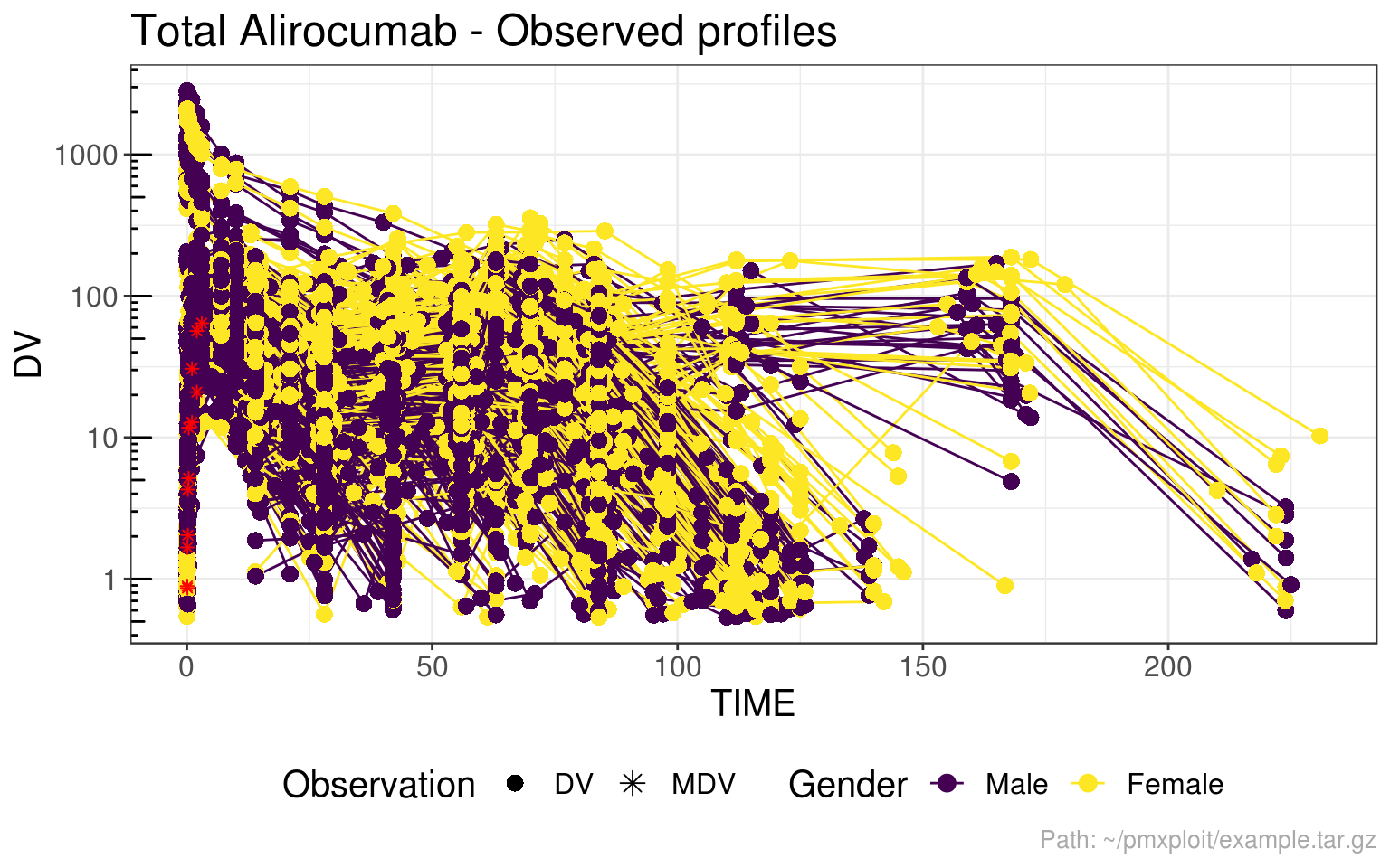

Dependent variable observations vs predictions

plot_dv_vs_predictions(run, compartment = 2, predictions = c("PRED", "IPRED"))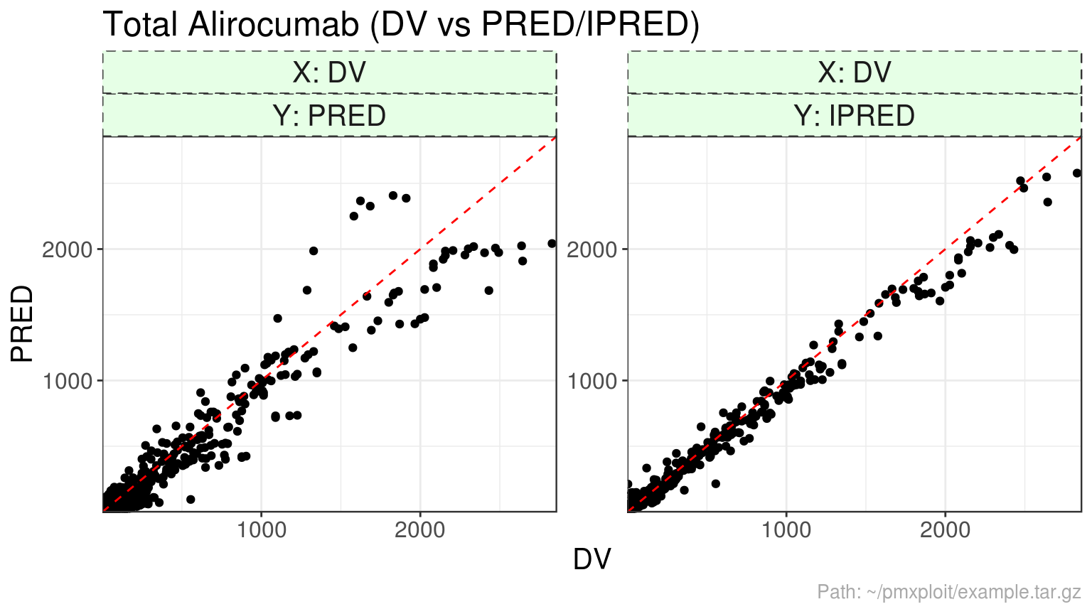

plot_dv_vs_predictions(run, compartment = 2, predictions = c("PRED", "IPRED"), x_scale = "log", y_scale = "log")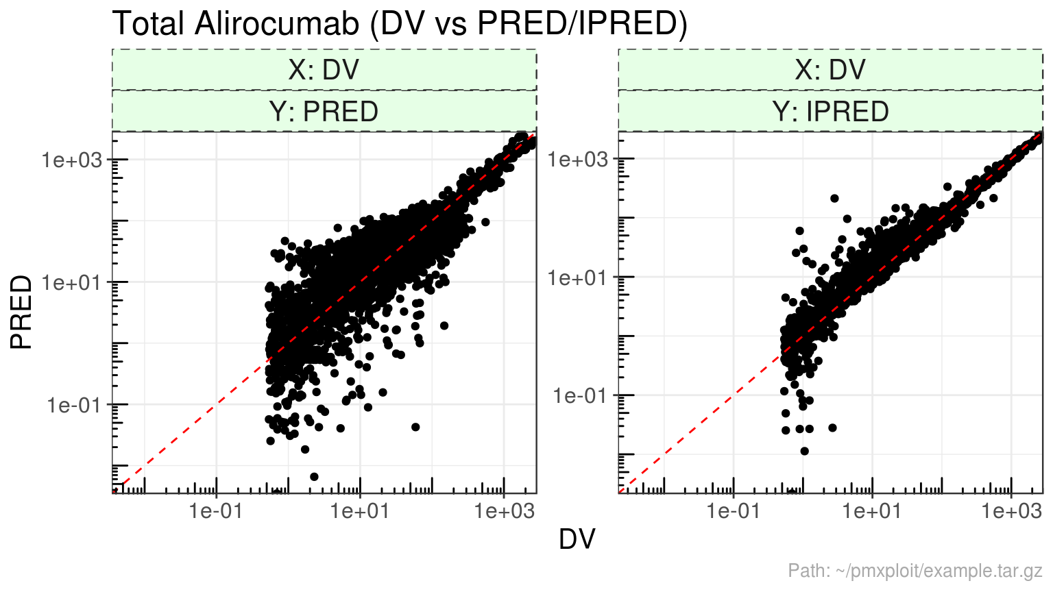

Residuals

plot_residuals(run, compartment = 2, residuals = "CWRES", idv = c("PRED", "TIME"), reference_value = 2)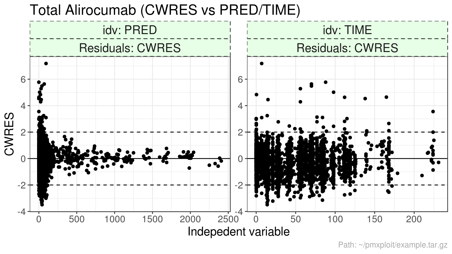


plot_residuals(run, compartment = 2, residuals = c("CWRES"), type = "histogram")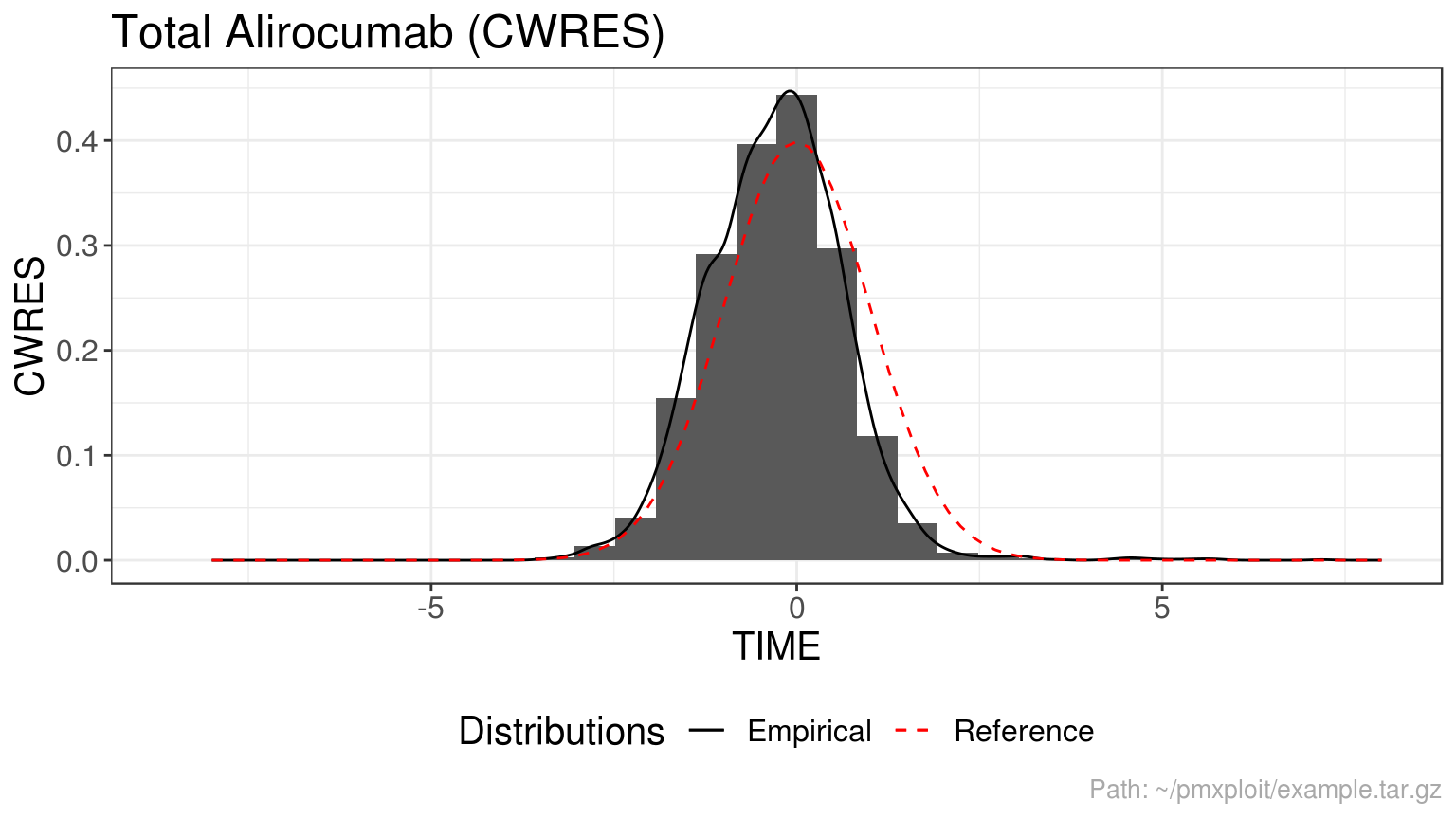

Individual predictions profiles

plot_individual_profiles(run, compartment = 2, ids = 1:4, predictions = c("PRED", "IPRED"), y_scale = "log")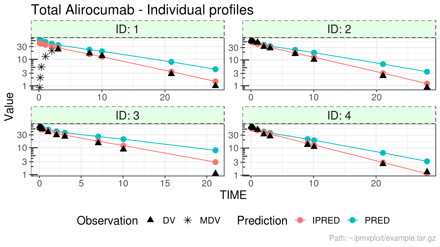

Population parameters

THETA

last_estimation <- last(run$estimations)

last_estimation$thetas %>% 
  mutate(rse = scales::percent(rse)) %>% 
  kable()

id	name	estimate	se	rse	ci_low	ci_up
THETA1	TVCL	0.1718969	0.0152002	8.84%	0.1414965	0.2022974
THETA2	TKON	559.0000000	NA	NA%	NA	NA
THETA3	TKIN	0.1238032	0.0022245	1.80%	0.1193541	0.1282523
THETA4	TKDE	1.3463553	0.0375067	2.79%	1.2713418	1.4213687
THETA5	TVQ	0.5003945	0.0285826	5.71%	0.4432292	0.5575597
THETA6	TVV1	3.2259046	0.2038901	6.32%	2.8181244	3.6336848
THETA7	TVV2	2.6120000	NA	NA%	NA	NA
THETA8	TVKA	0.6377794	0.0467722	7.33%	0.5442350	0.7313237
THETA9	TVF	0.5900018	0.0239372	4.06%	0.5421275	0.6378761
THETA10	TVEP	0.2746841	0.0015050	0.55%	0.2716741	0.2776941
THETA11	TVEA	0.5817956	0.0223812	3.85%	0.5370331	0.6265581
THETA12	TVLAG	0.0298266	0.0010994	3.69%	0.0276277	0.0320255
THETA13	COV1	1.5642857	0.0850631	5.44%	1.3941594	1.7344120

Convergence

plot_convergence(run, parameters = "theta")
#> Not shown fixed parameter(s): TKON, TVV2

OMEGA

# OMEGA matrix
kable(last_estimation$omega_matrix)

	ETCL	EKIN	EKDE	ETQ	ETV1	ETKA	ETF
ETCL	0.279196	0.0000000	0.0000000	0.0000000	0.000000	0.0000000	0.0000000
EKON	0.000000	0.0000000	0.0000000	0.0000000	0.000000	0.0000000	0.0000000
EKIN	0.000000	0.0580908	0.0000000	0.0000000	0.000000	0.0000000	0.0000000
EKDE	0.000000	0.0000000	0.1705345	0.0000000	0.000000	0.0000000	0.0000000
ETQ	0.000000	0.0000000	0.0000000	0.0691066	0.000000	0.0000000	0.0000000
ETV1	0.000000	0.0000000	0.0000000	0.0000000	0.099037	0.0000000	0.0000000
ETV2	0.000000	0.0000000	0.0000000	0.0000000	0.000000	0.0000000	0.0000000
ETKA	0.000000	0.0000000	0.0000000	0.0000000	0.000000	0.4644621	0.0000000
ETF	0.000000	0.0000000	0.0000000	0.0000000	0.000000	0.0000000	0.2895511


# OMEGA matrix as a table, with RSE% and IC 95%
last_estimation$omega %>% 
  mutate(rse = scales::percent(rse)) %>% 
  kable()

eta1	eta2	estimate	se	rse	ci_low	ci_up	cv
ETCL	ETCL	0.2791960	0.0761155	27.3%	0.1300096	0.4283823	0.5675090
EKIN	EKIN	0.0580908	0.0046239	8.0%	0.0490280	0.0671536	0.2445633
EKDE	EKDE	0.1705345	0.0164141	9.6%	0.1383628	0.2027062	0.4312059
ETQ	ETQ	0.0691066	0.0297647	43.1%	0.0107678	0.1274454	0.2674891
ETV1	ETV1	0.0990370	0.0165851	16.7%	0.0665301	0.1315438	0.3226563
ETKA	ETKA	0.4644621	0.0494723	10.7%	0.3674963	0.5614279	0.7688681
ETF	ETF	0.2895511	0.0717353	24.8%	0.1489500	0.4301522	0.5795064

Shrinkage

last_estimation$shrinkage %>% 
  mutate(shrinkage = scales::percent(shrinkage)) %>% 
  kable()

Individuals

Parameters

Distributions

summarize_parameters_distributions(run)
#> # A tibble: 11 x 12
#>    parameter     n n_distinct    mean  median      sd  `5.0%` `25.0%`
#>    <fct>     <int>      <int>   <dbl>   <dbl>   <dbl>   <dbl>   <dbl>
#>  1 CL          527        493 1.68e-1 1.72e-1 3.05e-2 1.15e-1 1.58e-1
#>  2 KON         527          1 5.59e+2 5.59e+2 0.      5.59e+2 5.59e+2
#>  3 KSS         527         33 5.80e-1 5.80e-1 4.68e-5 5.80e-1 5.80e-1
#>  4 KINT        527        507 1.29e-1 1.25e-1 2.62e-2 9.35e-2 1.13e-1
#>  5 KDEG        527        520 1.38e+0 1.37e+0 4.46e-1 7.78e-1 1.09e+0
#>  6 Q           527        500 5.03e-1 5.00e-1 3.30e-2 4.65e-1 4.92e-1
#>  7 V1          527        523 4.59e+0 4.61e+0 1.30e+0 2.71e+0 3.54e+0
#>  8 V2          527          1 2.61e+0 2.61e+0 0.      2.61e+0 2.61e+0
#>  9 KA          527        496 6.53e-1 6.38e-1 2.52e-1 3.54e-1 5.62e-1
#> 10 ALAG1       527          1 2.98e-2 2.98e-2 0.      2.98e-2 2.98e-2
#> 11 F1          527        494 6.08e-1 5.95e-1 1.20e-1 4.62e-1 5.42e-1
#> # … with 4 more variables: `75.0%` <dbl>, `95.0%` <dbl>, min <dbl>,
#> #   max <dbl>

plot_parameters_distributions(run, parameters = "eta")
#> Warning: Computation failed in `stat_bin()`:
#> `binwidth` must be positive

#> Warning: Computation failed in `stat_bin()`:
#> `binwidth` must be positive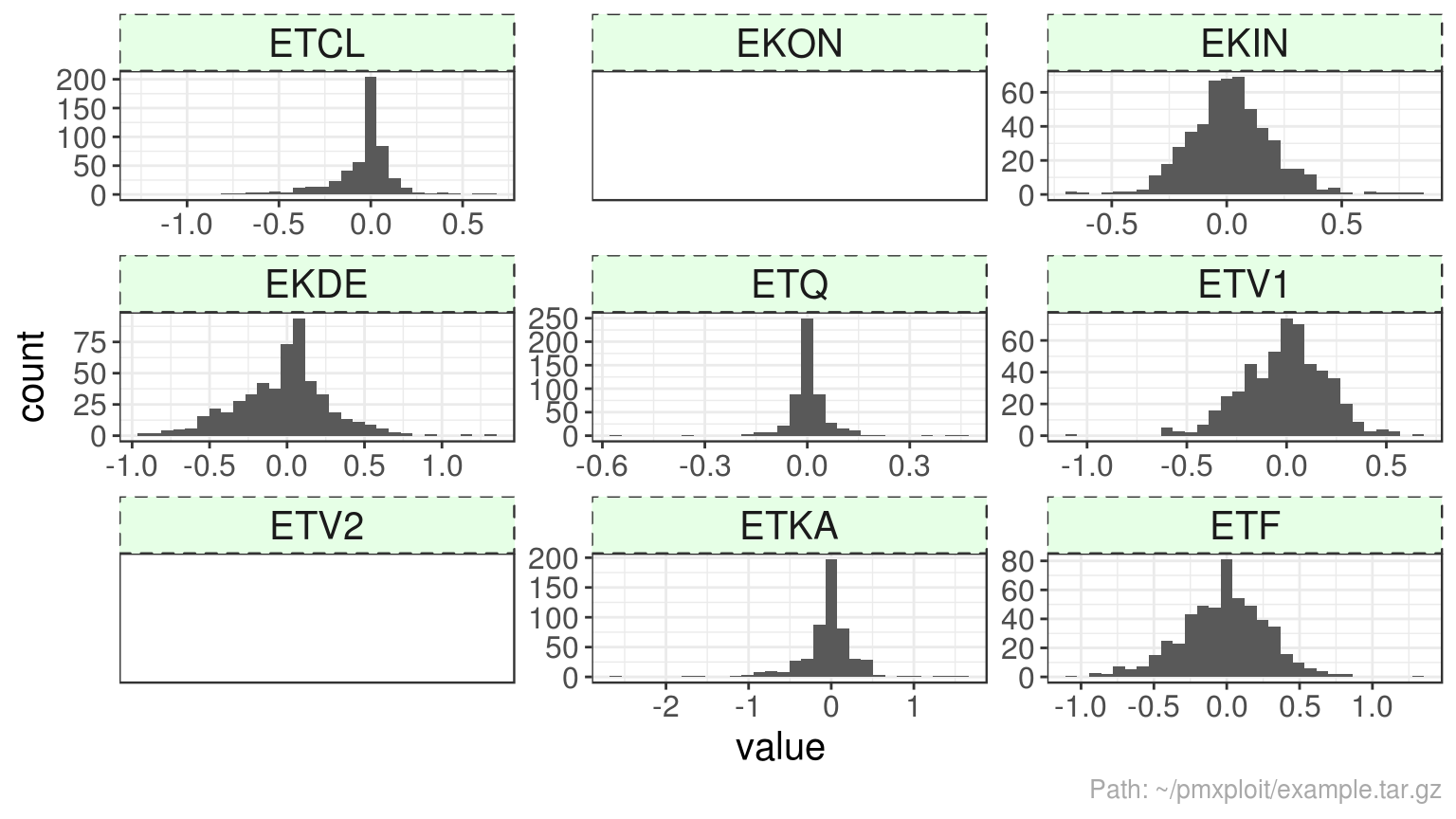


run %>% 
  group_by(STUD) %>%
  plot_parameters_distributions(parameters = c("CL", "V1"), type = "boxplot")

Correlations

summarize_parameters_correlations(run, parameters = "individual")
#> Correlations are not computed for parameters(s) with one unique value: KON, V2, ALAG1
#>               V1          F1           Q       KSS      KINT          KA
#> V1    1.00000000 -0.58741001 -0.05479555 0.1106159 0.1098006  0.30323370
#> F1   -0.58741001  1.00000000  0.13141825 0.2147780 0.2165945 -0.06226802
#> Q    -0.05479555  0.13141825  1.00000000 0.3817025 0.3792538  0.05201759
#> KSS   0.11061590  0.21477798  0.38170253 1.0000000 0.9981868  0.19737220
#> KINT  0.10980058  0.21659448  0.37925379 0.9981868 1.0000000  0.19826681
#> KA    0.30323370 -0.06226802  0.05201759 0.1973722 0.1982668  1.00000000
#> CL    0.30095621  0.02300692  0.09799981 0.3480292 0.3480398  0.22345707
#> KDEG  0.16623895 -0.04360299  0.09469923 0.2157855 0.2162849  0.17495309
#>              CL        KDEG
#> V1   0.30095621  0.16623895
#> F1   0.02300692 -0.04360299
#> Q    0.09799981  0.09469923
#> KSS  0.34802922  0.21578546
#> KINT 0.34803981  0.21628493
#> KA   0.22345707  0.17495309
#> CL   1.00000000  0.33390241
#> KDEG 0.33390241  1.00000000

plot_parameters_correlations(run, parameters = "eta", type = "heatmap")
#> Correlations are not computed for parameters(s) with one unique value: EKON, ETV2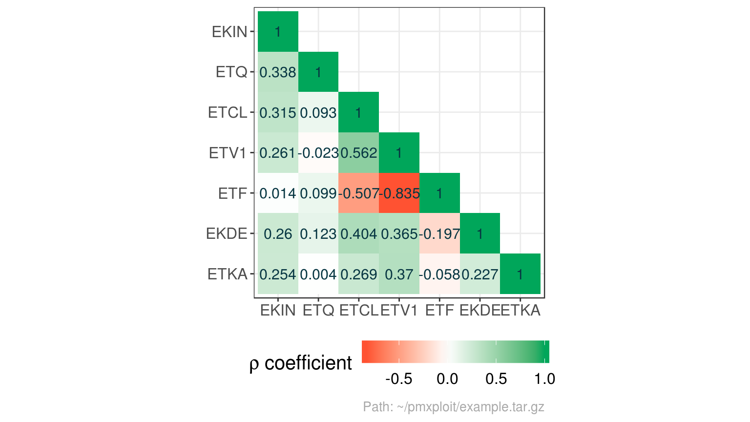

Continuous covariates

Distributions

summarize_continuous_covariates(run)
#> # A tibble: 8 x 12
#>   covariate     n n_distinct   mean median    sd `5.0%` `25.0%` `75.0%`
#>   <fct>     <int>      <int>  <dbl>  <dbl> <dbl>  <dbl>   <dbl>   <dbl>
#> 1 Age (y)     527         58  52.5   56    13.0   24      46      62   
#> 2 BMI (kg/…   527        438  28.0   27.4   4.60  21.5    24.7    30.7 
#> 3 Baseline…   527        320 140.   134.   33.0  101     117.    157.  
#> 4 Creatini…   527        517 109.   104.   30.4   67.6    87.3   128.  
#> 5 Baseline…   527        291   2.55   2.39  1.07   1.22    1.81    3.08
#> 6 Glomerul…   527        480  94.1   90.8  21.1   66.6    79.6   105.  
#> 7 Baseline…   527        437   7.66   6.99  3.06   3.73    5.61    9.14
#> 8 Weight (…   527        345  80.6   79.2  16.4   57.3    69.0    89.4 
#> # … with 3 more variables: `95.0%` <dbl>, min <dbl>, max <dbl>

plot_continuous_covariates_distributions(run)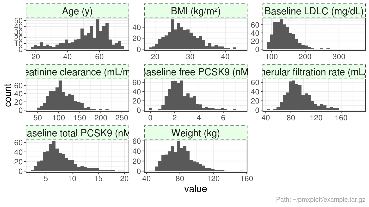

run %>% 
  group_by(STUD) %>%
  plot_continuous_covariates_distributions(type = "boxplot")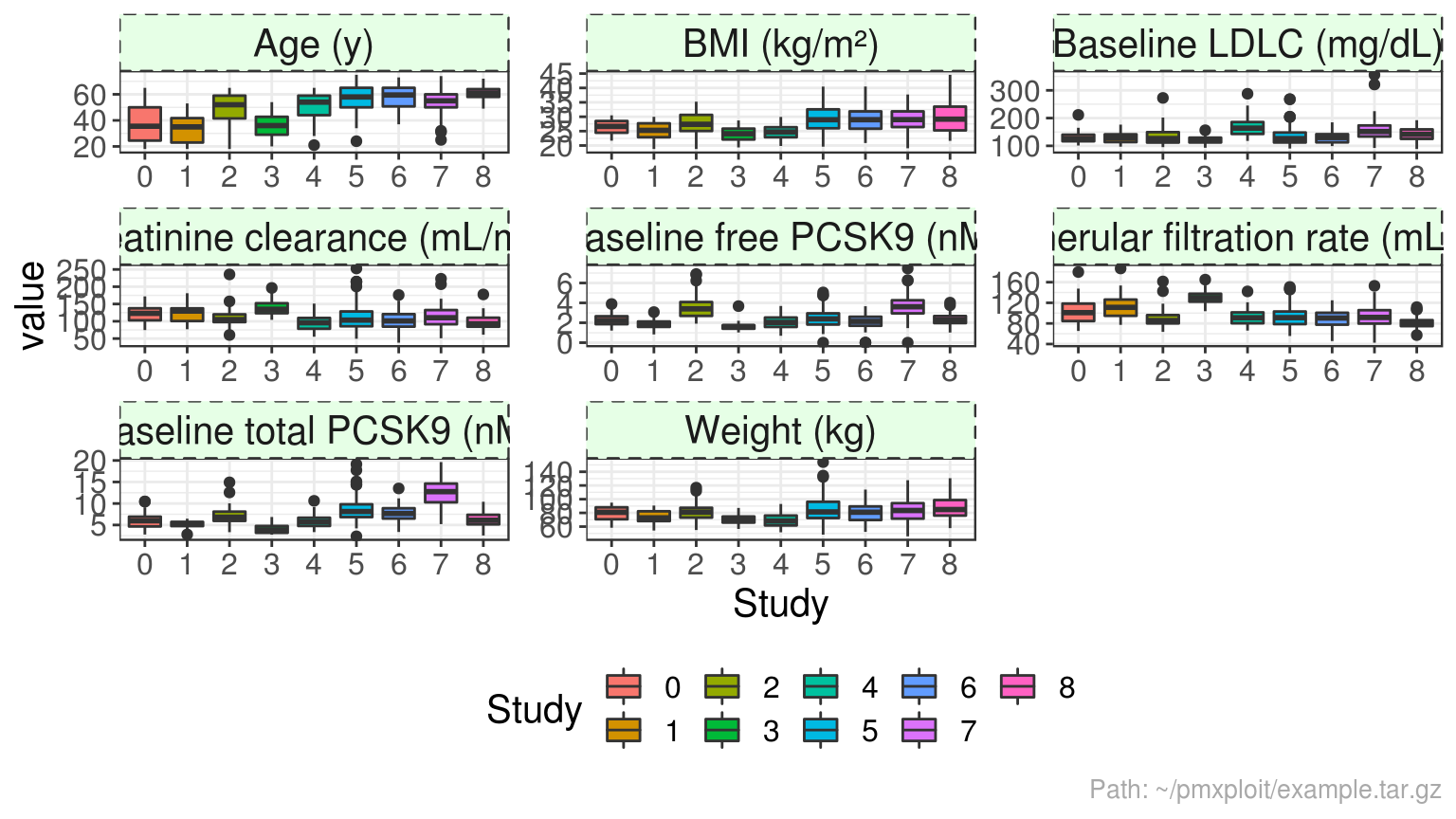

Correlations

summarize_covariates_correlations(run)
#>                                     Baseline free PCSK9 (nM)
#> Baseline free PCSK9 (nM)                          1.00000000
#> Baseline total PCSK9 (nM)                         0.63474111
#> Creatinine clearance (mL/min)                    -0.03390245
#> Age (y)                                           0.11602376
#> Glomerular filtration rate (mL/min)              -0.13572416
#> Baseline LDLC (mg/dL)                            -0.05890704
#> BMI (kg/m²)                                       0.14352343
#> Weight (kg)                                       0.10401265
#>                                     Baseline total PCSK9 (nM)
#> Baseline free PCSK9 (nM)                           0.63474111
#> Baseline total PCSK9 (nM)                          1.00000000
#> Creatinine clearance (mL/min)                     -0.06800086
#> Age (y)                                            0.26465204
#> Glomerular filtration rate (mL/min)               -0.14715975
#> Baseline LDLC (mg/dL)                              0.12308252
#> BMI (kg/m²)                                        0.17724420
#> Weight (kg)                                        0.08670552
#>                                     Creatinine clearance (mL/min)
#> Baseline free PCSK9 (nM)                              -0.03390245
#> Baseline total PCSK9 (nM)                             -0.06800086
#> Creatinine clearance (mL/min)                          1.00000000
#> Age (y)                                               -0.52845720
#> Glomerular filtration rate (mL/min)                    0.67538184
#> Baseline LDLC (mg/dL)                                 -0.12739227
#> BMI (kg/m²)                                            0.40805133
#> Weight (kg)                                            0.56597426
#>                                         Age (y)
#> Baseline free PCSK9 (nM)             0.11602376
#> Baseline total PCSK9 (nM)            0.26465204
#> Creatinine clearance (mL/min)       -0.52845720
#> Age (y)                              1.00000000
#> Glomerular filtration rate (mL/min) -0.51708487
#> Baseline LDLC (mg/dL)                0.01378944
#> BMI (kg/m²)                          0.20298742
#> Weight (kg)                          0.06328087
#>                                     Glomerular filtration rate (mL/min)
#> Baseline free PCSK9 (nM)                                    -0.13572416
#> Baseline total PCSK9 (nM)                                   -0.14715975
#> Creatinine clearance (mL/min)                                0.67538184
#> Age (y)                                                     -0.51708487
#> Glomerular filtration rate (mL/min)                          1.00000000
#> Baseline LDLC (mg/dL)                                       -0.03312037
#> BMI (kg/m²)                                                 -0.15911903
#> Weight (kg)                                                 -0.10956357
#>                                     Baseline LDLC (mg/dL) BMI (kg/m²)
#> Baseline free PCSK9 (nM)                      -0.05890704   0.1435234
#> Baseline total PCSK9 (nM)                      0.12308252   0.1772442
#> Creatinine clearance (mL/min)                 -0.12739227   0.4080513
#> Age (y)                                        0.01378944   0.2029874
#> Glomerular filtration rate (mL/min)           -0.03312037  -0.1591190
#> Baseline LDLC (mg/dL)                          1.00000000  -0.1510291
#> BMI (kg/m²)                                   -0.15102914   1.0000000
#> Weight (kg)                                   -0.16168067   0.7920918
#>                                     Weight (kg)
#> Baseline free PCSK9 (nM)             0.10401265
#> Baseline total PCSK9 (nM)            0.08670552
#> Creatinine clearance (mL/min)        0.56597426
#> Age (y)                              0.06328087
#> Glomerular filtration rate (mL/min) -0.10956357
#> Baseline LDLC (mg/dL)               -0.16168067
#> BMI (kg/m²)                          0.79209179
#> Weight (kg)                          1.00000000

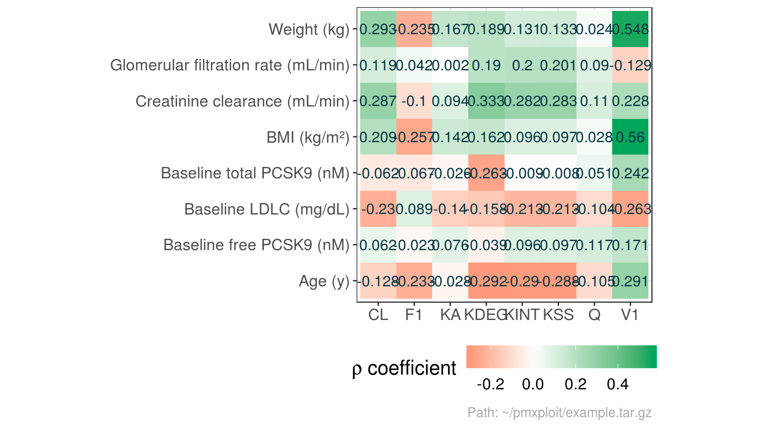
plot_covariates_correlations(run, type = "heatmap")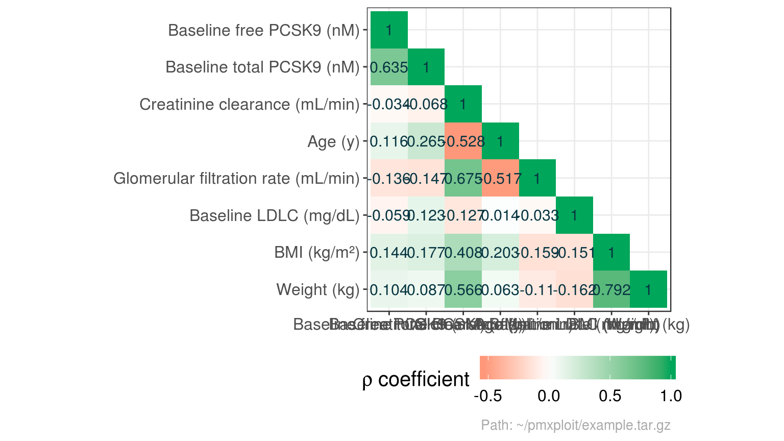


run %>% 
  group_by(STUD) %>%
  plot_covariates_correlations(type = "scatterplot")
#> Warning in GGally::ggscatmat(as.data.frame(select(df, -ID))): Factor
#> variables are omitted in plot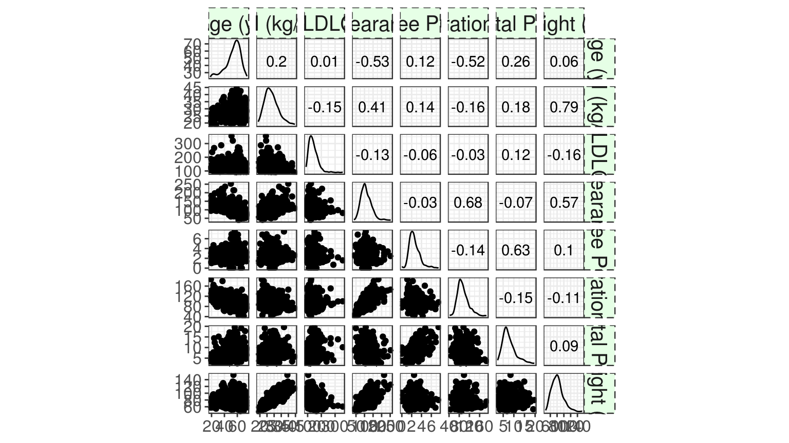

Parameters vs covariates

plot_parameters_vs_continuous_covariates(run)


plot_parameters_vs_categorical_covariates(run, parameters = c("CL", "V1"))

Quality criteria

# Overall QC
qc <- quality_criteria(run, predictions = "PRED")

# QC by study
qc_stud <- run %>% 
  group_by(STUD) %>%
  quality_criteria(predictions = "PRED")

kable(qc$standard)

max_err	aafe
786.5671	1.566821


qc_stud %>% 
  select(Study, standard) %>% 
  unnest() %>% 
  kable()

Study	max_err	aafe
0	786.5671	1.402490
1	120.9971	1.487727
2	171.3205	1.516194
3	113.7925	1.569381
4	460.8415	1.550188
5	190.3589	1.605442
6	117.1923	1.637036
7	228.3282	1.624440
8	146.0201	1.847918


# Bias
qc_stud %>% 
  select(Study, bias) %>% 
  unnest() %>% 
  mutate(relative_value = scales::percent(relative_value)) %>% 
  rename(`Mean Prediction Error (%)` = relative_value) %>% 
  kable()

Study	value	ci_low	ci_up	Mean Prediction Error (%)
0	-14.2811313	-22.301736	-6.260527	-5.8%
1	0.4946943	-1.185524	2.174913	1.8%
2	-4.1641145	-4.904954	-3.423276	-18.4%
3	8.4579500	6.735203	10.180697	25.3%
4	-10.8373662	-12.183189	-9.491543	-22.2%
5	1.9028940	1.002670	2.803118	5.9%
6	-0.3312528	-2.009636	1.347131	-0.9%
7	-9.5851697	-11.691082	-7.479257	-20.6%
8	-13.3829373	-15.581440	-11.184434	-31.6%


# Precision
qc_stud %>% 
  select(Study, precision) %>% 
  unnest() %>% 
  mutate(relative_value = scales::percent(relative_value)) %>% 
  rename(`Root Mean Square Error (%)` = relative_value) %>% 
  kable()

Study	value	ci_low	ci_up	Root Mean Square Error (%)
0	119.60062	101.32976	135.42856	48.9%
1	19.36620	16.31571	21.99766	71.3%
2	16.07381	14.11605	17.81773	71.2%
3	22.88012	20.21317	25.26712	68.4%
4	30.11989	24.73595	34.67777	61.7%
5	20.95346	19.33192	22.45822	65.5%
6	21.78440	19.38433	23.94509	56.7%
7	33.23176	28.39221	37.45106	71.5%
8	28.31826	24.68632	31.53464	66.8%

Introduction to pmxploit

Patrick Nolain

2019-02-26

Load a NONMEM run archive

Job details

Run information

Model/Data/Files

Estimation

Model information

Compartments

Parameters

Covariates

Diagnostic plots

Spaghetti plot

Dependent variable observations vs predictions

Residuals

Individual predictions profiles

Population parameters

THETA

Convergence

OMEGA

Shrinkage

Individuals

Parameters

Distributions

Correlations

Continuous covariates

Distributions

Correlations

Parameters vs covariates

Quality criteria

Contents